Daytime length variations with latitude and season (1/3)
It is easy to explain the changing seasons and the variation in the length of day and night time at different latitudes by means of the axial tilt, also known as obliquity (Wikipedia (n.d.a)).
Earth currently has a mean tilt of 23.44° (Wikipedia (n.d.a)) between:
- its rotational axis, the imaginary line that passes through both poles, and on which Earth spins producing the 24-hour day,
- and its orbital axis, the line perpendicular to the imaginary plane (ecliptic) across which Earth moves as it revolves around the Sun, producing the 365-day year.
The figure 1 shows the two axes and the axial tilt between them.
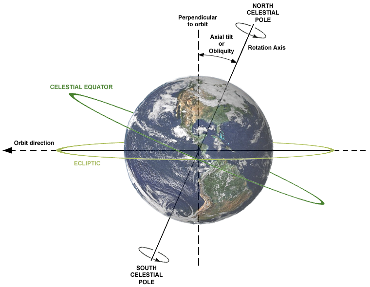
Figure 1: Axial Tilt, By I, Dennis Nilsson, CC BY 3.0, https://commons.wikimedia.org/w/index.php?curid=3262268
Over the course of a revolution around the Sun, the orientation of the rotational axis remains the same respect to the background of distant stars. As a result, the orientation of the rotaxional axis relative to the Sun varies along the Earth’s orbit.
The figure 2 shows the orientation of the rotational axis in two opposite points of the Earth’s orbit, on June solstice and December solstice, when the tilt of the rotational axis is at its maximum, toward the Sun or away from the Sun.
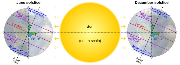
Figure 2: Axis Orientation in opposite points of the Earth’s orbit, By cmglee, NASA - Own work using: http://visibleearth.nasa.gov/view.php?id=73580, Public Domain, https://commons.wikimedia.org/w/index.php?curid=41309095
This post is the first of a series that explores how to calculate and visualize the daytime length by latitude and day in the year using R.
Simple model
A simple model has been built upon the concepts described above. The most relevant approximations in the model are listed below together with a short note qualifying to what extent deviates from the reality.
- Earth is modelled like a sphere. In fact, Earth is only approximately spherical, it deviates mainly due to the centrifugal force caused by its rotation (Wikipedia, n.d.c) and, to a lesser extent, to its non-uniform density and geological phenomena.
- Earth spins on its own axis (the rotational axis) once every 24 hours. Earth’s rotational period is not constant mainly due to the tidal forces of the Moon (Wikipedia, n.d.b).
- Earth revolves about the Sun in a circular orbit once every 365 days. Celestial orbits are not perfectly circular. While Earth’s orbit is better approximated by an ellipse, the influence of the other solar system bodies continously alters its orbit.
- Earth’s motion is decomposed in an intertwined succession of discrete rotations and translations (revolution): rotates, revolves, rotates, revolves … Earth’s motion is continous, it spins as it revolves.
- The axial tilt is 23.44° and remains the same over an orbital period. The axial tilt oscillates between 22.1° and 24.5° on a 41,000-year cycle (Wikipedia (n.d.a)).
- Parallel sunlight. The Sun and the Earth are so far apart that the sunlight appears to be parallel on Earth. Check this animation to get a feeling of how good is this approximation.
- At any time, half of the Earth is illuminated by the Sun and the other half is at night. This removes the necessity of modelling the Sun at all. This is a result of simplifications 1) and 6).
- The effect of the atmospheric refraction is negligible in the day- and nightime. The refraction may make the sun visible for several minutes before it raises and after it sets (Konstantin Bikos, n.d.).
Conventions
The figure 3 depicts the conventions in relation with the system coordinates followed in the series.
- x-axis and y-axis make up the horizontal plane
- z-axis is always the vertical axis and is positive upwards.
- The polar coordinate \(\theta\) is measured from the z-axis (positive pointing upwards).
- Rotation follows the right-hand rule, when the thumb is pointing in the positive direction along the axis of rotation, then the curled fingers indicate the positive rotation direction.

Figure 3: Cartesian and polar coordinates, By Andeggs - Own work, Public Domain, https://commons.wikimedia.org/w/index.php?curid=7478049
Grid generation
The first step is the generation of points to model Earth, these points are then used to determine the daytime length at different latitudes at different times in the year.
The grid is determined by the following parameters:
Latitude points
Set of angles raging from -90° (South Pole) to 90° (North Pole), 0° at the Equator. The number of latitude points is controlled by the parameter lat_step. The parameter is set to 10, resulting in 19 latitudes, to keep a manageable number of points and a resonable time for rendering the plots. The value of the step can be reduced to increase the number of points and the resolution.
1lat_step <- 10
2lat_pts <- seq(from = - 90, to = 90, by = lat_step)
3num_lat_pts <- length(lat_pts)
Calculating latitude points
The polar coordinate \(\theta\) can be determined from the latitude in degrees using the following formula: \(\theta (rad) = {\pi \over 2} \times { (1 - {latidude (degrees) \over 90})}\)
Once we have the angle \(\theta\), the cartesian coordinates may be retrieved from the spherical coordinates by the following equations:
- \(x = r \times cos(\varphi) \times sin(\theta)\)
- \(y = r \times sin(\varphi) \times sin(\theta)\)
- \(z = r \times cos(\theta)\)
Thus, for \(r = 1\)
1coor_lat <- matrix(1, num_lat_pts, 3)
2x_lat <- sin( pi / 2 * (1 - lat_pts / 90))
3y_lat <- sin( pi / 2 * (1 - lat_pts / 90))
4z_lat <- cos( pi / 2 * (1 - lat_pts / 90))
5coor_lat[,1] <- x_lat
6coor_lat[,2] <- y_lat
7coor_lat[,3] <- z_lat
8colnames(coor_lat) <- c('x', 'y', 'z')
… and \(\varphi = 0\) the figure 4 plots in 3D the resulting latitude points using the library plotly.
- \(x = r \times sin(\theta)\)
- \(y = 0\)
- \(z = r \times cos(\theta)\)
1scene = list(camera = list(eye = list(x = 0, y = 2, z = 0)))
2fig_lat <- plot_ly() %>% config(displayModeBar = FALSE, scrollZoom = FALSE)
3fig_lat <- fig_lat %>% add_trace(data = coor_lat, x = coor_lat[,'x'], y = 0, z = coor_lat[,'z'], type ='catter3d', mode='markers', size=1) %>% layout(scene = scene)
4fig_lat
Figure 4: Latitude points
Points along the parallel (longitude)
Set of angles into which a parallel (line of constant latitude) circling the Earth is divided. To simplify the calculation of the daytime length later in this series it ranges from 1 to 48 (multiple of 24).
The number of points is controlled by the parameter lon_step. The parameter is set to 1, resulting in 48 points for each parallel.
1lon_step <- 1
2lon_pts <- seq(from = 1, to = 48, by = lon_step)
3num_lon_pts <- length(lon_pts)
Calculating points on the Earth’s surface
For each latitude point a parallel line consisting of num_lon_pts is created. Therefore Earth´s surface is represented by num_lat_pts * num_lon_pts points of its spherical surface.
In order to do this, each latitude point is repeated num_lon_pts times. The \(cos(\varphi)\) and \(sin(\varphi)\) factors required to build a cicle are generated from the set of points along the parallel and applied to x and y coordinates for each latitude according to:
- \(x = r \times cos(\varphi) \times sin(\theta)\)
- \(y = r \times sin(\varphi) \times sin(\theta)\)
This code shows a very efficient way of doing it by using the function rep.
1coor_lat_lon <- matrix( rep( coor_lat, each = num_lon_pts), (num_lat_pts * num_lon_pts), 3)
2colnames(coor_lat_lon) <- c('x', 'y', 'z')
3coor_lat_lon[,'x'] <- coor_lat_lon[,'x'] * rep( cos( lon_pts * 2 * pi / num_lon_pts), num_lat_pts)
4coor_lat_lon[,'y'] <- coor_lat_lon[,'y'] * rep( sin( lon_pts * 2 * pi / num_lon_pts), num_lat_pts)
The figure 5 plots the resulting points.
1scene = list(camera = list(eye = list(x = 0, y = 2, z = 0)))
2fig_lat_lon <- plot_ly() %>% config(displayModeBar = FALSE, scrollZoom = FALSE)
3fig_lat_lon <- fig_lat_lon %>% add_trace(data = coor_lat_lon, x = coor_lat_lon[,'x'], y = coor_lat_lon[,'y'], z = coor_lat_lon[,'z'], type ='scatter3d', mode='markers', size=1) %>% layout(scene = scene)
4fig_lat_lon
Figure 5: Latitude and Longitude points
Year points
Set of points in the Earth’s orbit around the Sun. Each point represents a day in the year, or equivalently the position in Earth’s orbit on that day. These points are used to determine the orientation of the Earth’s rotational axis relative to the Sun on different days in the year.
The year points are controlled by the parameter year_step. The parameter is set to 15 to keep a manageable number of points and a resonable time for rendering the plots. The value of the step can be reduced to increase the number of points and the resolution.
1year_step <- 15
2year_pts <- seq(from = 1, to = 365, by = year_step)
3num_year_pts <- length(year_pts)
Rotations
Next I compile the basic rotation matrices in 3D by an angle θ about the different axes: x-(1) , y-(2), or z-axis(3):
\[\begin{equation} R_x(\theta) = \begin{pmatrix} 1 & 0 & 0 \\ 0 & cos \theta & -sin \theta \\ 0 & sin \theta & cos \theta \end{pmatrix} \tag{1} \end{equation}\]
\[\begin{equation} R_y(\theta) = \begin{pmatrix} cos \theta & 0 & sin \theta \\ 0 & 0 & 1 \\ sin \theta & cos \theta & 0 \end{pmatrix} \tag{2} \end{equation}\]
\[\begin{equation} R_z(\theta) = \begin{pmatrix} cos \theta & -sin \theta & 0 \\ sin \theta & cos \theta & 0 \\ 0 & 0 & 1 \end{pmatrix} \tag{3} \end{equation}\]
Theta represents here any angle and not the polar coordinate.
Axist tilt
The axis tilt is a rotation around the x-axis. Following the convention outlined earlier, the sign of this rotation is negative, thus the formula \(-23.44 \times 2\pi \over 360\).
Rotation follows the right-hand rule, when the thumb is pointing in the positive direction along the axis of rotation, then the curled fingers indicate the positive rotation direction.
1axis_tilt <- -23.44 * 2 * pi / 360
2rot_tilt_x <- matrix (c(1,0,0,0,cos(axis_tilt), -sin(axis_tilt),0, sin(axis_tilt), cos(axis_tilt)), 3,3)
3coor_lat_lon_tilt <- t(rot_tilt_x %*% t(coor_lat_lon))
4colnames(coor_lat_lon_tilt) <- c('x', 'y', 'z')
5scene = list(camera = list(eye = list(x = -2, y = 0, z = 0)))
6fig_lat_lon_tilt <- plot_ly() %>% config(displayModeBar = FALSE,  scrollZoom = FALSE)
7fig_lat_lon_tilt <- fig_lat_lon_tilt %>% add_trace(data = coor_lat_lon_tilt, x = coor_lat_lon_tilt[,'x'], y = coor_lat_lon_tilt[,'y'], z = coor_lat_lon_tilt[,'z'], type ='scatter3d', mode='markers', size=1) %>% layout(scene = scene)
8fig_lat_lon_tilt
The figure 6 plots the inclination of the rotational axis.
Figure 6: Axis tilt
Orientation of the rotational axis on different days in the year (orbital period)
The orientation of the Earth’s rotational axis relative to the Sun on different days in the year can be represented as a rotation around the z-axis (orbital axis).
The angle of the rotation depends on the number of year points and results of dividing the circle (\(2\pi\) rad) by the number of points.
In addition, an offset is calculated so that the relative orientation on the day 1 coincides with the orientation on the January 1st, this will help in interpreting the results when presented on a timeline.
1year_delta_ang <- year_step/365 * 2 * pi
2year_offset <- 175/365 * 2 * pi + year_delta_ang
3rot_year <- matrix (c(cos(year_delta_ang ), sin(year_delta_ang ),0, -sin(year_delta_ang ), cos(year_delta_ang) , 0,0,0,1), 3,3)
4rot_year_offset <- matrix (c(cos(year_offset ), sin(year_offset ),0, -sin(year_offset), cos(year_offset) , 0,0,0,1), 3,3)
For each year point, the points representing the sphere are rotated about the z-axis, the rotation is accumulated so that the next interation rotates till the next position until it completes the entire circle on the last day.
Avoid at any cost expanding a dataframe (rbind) within a loop in R, otherwise you will see yourself trapped in the second circle of R Hell.
Watch out that the points representing the sphere for each position are stored on its own dataframe and added to a list. The list of dataframes is later combined through rbindlist.
In my case, by doing so, the processing time went down from over 30 hours to barely 1 minute, you do not have to believe me, try it yourself.
 1df <- data.frame()
 2list_of_df_i <- vector(mode = 'list', length = num_year_pts)
 3rot_year_acc <- rot_year_offset
 4for (i_day in 1:num_year_pts) {
 5    coor_lat_lon_tilt_year <- t( rot_year_acc %*% t(coor_lat_lon_tilt))
 6    rot_year_acc <-  rot_year %*% rot_year_acc
 7    dim(coor_lat_lon_tilt_year)
 8    colnames( coor_lat_lon_tilt_year) <- c('xp', 'yp', 'zp')
 9    list_of_df_i[[i_day]] <- data.frame(xp=coor_lat_lon_tilt_year[,'xp'], yp=coor_lat_lon_tilt_year[,'yp'], zp=coor_lat_lon_tilt_year[,'zp'], lon_pt = rep(lon_pts, num_lat_pts), day =  rep(year_pts[i_day], num_lat_pts * num_lon_pts), latitude = rep(lat_pts, each=num_lon_pts))
10
11}
12df <- rbindlist(list_of_df_i)
The animation 7 shows the changes in the orientation of the rotational axis relative to the Sun over a year.
1scene = list(camera = list(eye = list(x = 2, y = 0, z = 0)))
2fig3d <- plot_ly() %>%  config(displayModeBar = FALSE,  scrollZoom = FALSE)
3fig3d <- fig3d %>% add_trace(data = df, x = ~xp, y = ~yp, z = ~zp, frame = ~ day,type ='scatter3d', mode='markers', size=1 ) %>% layout(scene = scene)
4fig3d
Figure 7: Orientation of the rotational axis relative to the Sun over a year
Do not mistake this rotation around the z-axis that represents the orientation of the rotational axis relative to the Sun, with the 24-hour day rotation, the latter is around the rotational axis and not around the z-axis.
Stay tuned, in next post we will calculate the daytime length using the grid we have just built up.
References
Posts in this Series
- Daytime length variations with latitude and season (3/3)
- Daytime length variations with latitude and season (2/3)